-
Notifications
You must be signed in to change notification settings - Fork 5
split, merge, reformulate assembly_visualization.md #7
New issue
Have a question about this project? Sign up for a free GitHub account to open an issue and contact its maintainers and the community.
By clicking “Sign up for GitHub”, you agree to our terms of service and privacy statement. We’ll occasionally send you account related emails.
Already on GitHub? Sign in to your account
Open
evezeyl
wants to merge
4
commits into
dev
Choose a base branch
from
evfi_split_move_assembly_visualization
base: dev
Could not load branches
Branch not found: {{ refName }}
Loading
Could not load tags
Nothing to show
Loading
Are you sure you want to change the base?
Some commits from the old base branch may be removed from the timeline,
and old review comments may become outdated.
Open
Changes from all commits
Commits
Show all changes
4 commits
Select commit
Hold shift + click to select a range
862c926
split, merge, reformulate assembly_visualization.md
evezeyl 2e0279d
Merge branch 'master' of https://github.com/NorwegianVeterinaryInstit…
evezeyl 292770b
implemented suggested corrections
evezeyl 2221133
created transfering files: rsync osv - need to complete
evezeyl File filter
Filter by extension
Conversations
Failed to load comments.
Loading
Jump to
Jump to file
Failed to load files.
Loading
Diff view
Diff view
There are no files selected for viewing
This file contains hidden or bidirectional Unicode text that may be interpreted or compiled differently than what appears below. To review, open the file in an editor that reveals hidden Unicode characters.
Learn more about bidirectional Unicode characters
| Original file line number | Diff line number | Diff line change |
|---|---|---|
| @@ -0,0 +1,40 @@ | ||
| # Using a graphical window in SAGA | ||
| It is possible to use graphical interface on Saga. | ||
| Login to saga using the `-Y` option | ||
|
|
||
|
|
||
| _**PRACTICAL EXERCISE:**_ | ||
|
|
||
| ```bash | ||
| ssh -Y <username>@saga.sigma2.no | ||
| ``` | ||
|
|
||
| Do a simple test that to check that it is working | ||
|
|
||
| ```bash | ||
| xeyes | ||
| ``` | ||
|
|
||
| type `ctrl+C` to kill xeyes | ||
|
|
||
|
|
||
| You can read more on [SAGA manual: X11 forwarding](https://documentation.sigma2.no/getting_started/create_ssh_keys.html#x11-forwarding) | ||
|
|
||
|
|
||
| ## Concrete example | ||
| Below is an example where we are using IGV, which is required for the tutorial:[Visualizing assembly and associated reads pileup with IGV](../tutorials/Visualisation_assembly_reads_pileup_IGV.md) | ||
|
|
||
| Ask for ressources on Saga to use IGV (do not forget `--x11`) | ||
|
|
||
| ```bash | ||
| # Example of how to use the ressources interactively | ||
| srun --account=nn9305k --mem-per-cpu=16G --cpus-per-task=1 --qos=devel \ | ||
| --time=0:30:00 --x11 --pty bash -i | ||
| conda activate igv | ||
| # launching IGV | ||
| igv | ||
| ``` | ||
|
|
||
| A window with IVG should open. | ||
|
|
||
| You will see several error messages that it tries to load a genome file, ignore those (it is because there are some server data that try to be loaded through internet, but we have no internet access from the compute nodes. Anyway we do not need those data to work with.) |
Loading
Sorry, something went wrong. Reload?
Sorry, we cannot display this file.
Sorry, this file is invalid so it cannot be displayed.
67 changes: 67 additions & 0 deletions
67
docs/source/tutorials/Visualisation_assembly_reads_pileup_IGV.md
This file contains hidden or bidirectional Unicode text that may be interpreted or compiled differently than what appears below. To review, open the file in an editor that reveals hidden Unicode characters.
Learn more about bidirectional Unicode characters
| Original file line number | Diff line number | Diff line change |
|---|---|---|
| @@ -0,0 +1,67 @@ | ||
| # Visualizing assembly and associated reads pileup with IGV | ||
|
|
||
| The [IGV: Integrative Genomics Viewer](http://software.broadinstitute.org/software/igv/home) software allows to visually explore and scroll through sequences, that may or not be split in contigs, and may or not be associated with reads pileup. It can eg. allow you to detect specific positions were variants are erroneous (eg. at the end of contigs where reads are poorly mapped) and visualize eg. locations where coverage is not homogeneous (ie. repeated regions that are not proprely assembled). | ||
|
|
||
| NB: Convention: means `<change_me>` | ||
|
|
||
| ## 1. Access to IGV | ||
|
|
||
| - You can access [IGV online](https://igv.org/app/). If you use this solution **be aware that data might be accessible or become publicly aware as they are uploaded to the website**. | ||
| - You can install IGV on your own PC, this requires that your files are on the same machine (Please see <software.vetinst.no> for installation). | ||
| - You can use saga with a graphical user interface. Please see the techinical: [Using a graphical window in SAGA](../technical/Saga_graphical_interface.md). **For Mac and Linux users only**. Be aware that you can have a Virtual Machine (VM) installed on a Windows PC (eg. on Virtual Box), or can request a Bioinformatic computer with Linux installed. | ||
|
|
||
| ## 2. Example: using IGV with reads mapped to its own assembly | ||
|
|
||
| We have assembled reads and annotated using Bifrost pipeline. The data for the practical are found in `/cluster/projects/nn9305k/tutorial/20210412_mapping_visualization/visualisation_files` | ||
|
|
||
| Files description: | ||
| - the assembly (polished with Pilon, **output provided by Prokka annoation** ) is: `MiSeq_Ecoli_MG1655_50x.fna` (fasta format) | ||
| - the genome annotation is the file (.gff) provided by `Prokka` : `MiSeq_Ecoli_MG1655_50x.gff` | ||
| - the final `.bam` file: `final_all_merged.bam` that contained the mapping of the PE and Unpaired reads to the assembly (used as reference) | ||
| - A `.bed` file (or gap track): `MiSeq_Ecoli_MG1655.bed` that allows easily identification of scaffolds limits (gaps). | ||
|
|
||
| NB: you can see you to generate those files see the tutorial: [Mapping reads against a reference/assembly](./Visualisation_assembly_reads_pileup_IGV.md) and in the [Creating gap tracks](./creating_file_visualize_gaps.md) | ||
|
|
||
| If you work on your pc you want to transfer those files to a local folder. If in need, please look at the tutorial regarding [file transfer](./transfering_files.md) | ||
|
|
||
| Now you can load those files in [IGV](https://software.broadinstitute.org/software/igv/) | ||
|
|
||
|  | ||
|
|
||
|
|
||
| _**PRACTICAL EXERCISE:**_ | ||
|
|
||
| 1. Create a `genome file` this allows associating tracks to the assembly : `Genomes > create.genome file`. Use the menu to select your assembly file `.fasta`and the annotation-gene file: `.gff`. | ||
| A track corresponds to a row of information that is displayed in IGV (one track per type of information. Information provided to IGV by loading one file: eg. the mapping file, the genome/assembly file, the file representing gaps between scaffolds). | ||
|
|
||
| NB: You need to fill the `unique identifier` AND `descriptive name` fileds. | ||
|
|
||
| 2. Locate and Load your `mapped reads` and the `gap file` using: `file > load from file` | ||
| - if you use SAGA here: you need to navigate throught the file structure: cluster>projects>nn9305k>active> and your own folder | ||
|
|
||
| 3. To be able to easily re-open (without re-importing everything you can do): `file > save session` | ||
| - be carefull where you save in the navigator when using SAGA | ||
|
|
||
| Now you are ready to navigate and explore your assembly. | ||
|
|
||
| **Try to find a gap.** | ||
|
|
||
| NB: To zoom while staying centered on the gap: click above menu (position within the scaffold - at the gap - top track) then click with the mouse at the gap position on the gap track (until appropriate zoom is obtained). | ||
|
|
||
| You can look here for [Options and interpretation](http://software.broadinstitute.org/software/igv/PopupMenus#AlignmentTrack), | ||
| and here: [PE orientations](http://software.broadinstitute.org/software/igv/interpreting_pair_orientations). | ||
|
|
||
| **Have a look at:** | ||
| - coverage | ||
| - gaps positions | ||
| - some strange scaffolds? | ||
| - PE orientations: in detail how the reads map to your assembly (you will need to zoom a lot) | ||
| - are some PE reads miss-oriented? reported as having abnormal insert sizes? | ||
|
|
||
| ## Troubleshooting | ||
|
|
||
| To be able to link the positions in the assembly to the annotations, the scaffold names between assembly and annotations files have to be consistent when provided as input file into IGV. | ||
|
|
||
| This is why we used the assembly that prokka outputs in the present example (this is the sequence is the same as .fasta assembly polished by pilon). Indeed, `Prokka` transforms scaffold names from the assembly used as input. If scaffold names in the annotation file and sequence file are not consistent, IGV will not manage to link the information of both files. | ||
|
|
||
| If you encounter such case, and do not have access to the assembly provided by prokka, the solution is to use an alias file. The alias file will provide to IGV the correspondance between contigs of your sequence/assembly and the annotation file. This is [described here](https://software.broadinstitute.org/software/igv/LoadData/#aliasfile) |
This file contains hidden or bidirectional Unicode text that may be interpreted or compiled differently than what appears below. To review, open the file in an editor that reveals hidden Unicode characters.
Learn more about bidirectional Unicode characters
| Original file line number | Diff line number | Diff line change |
|---|---|---|
| @@ -0,0 +1,28 @@ | ||
| # Creating a file to visualize gaps in genomes | ||
|
|
||
| When you attempt to visualize genome assemblies with software such as IGV, beeing able to easily locate starting/and ending scaffold locations is very usefull. This, because those positions are potentially problematic regions of an assembly. A gap file (refered to as `.bed` file) provides the locations where scaffolds are interupted. Those file also also to rapidely navigate through the different scaffolds when provided to visualization softwares. | ||
|
|
||
|
|
||
| We use a little python script from [sequencetools repository](https://github.com/lexnederbragt/sequencetools) to create `bed`files. NB: If you use this script in an article you need to proprely aknowledge Lex Nederbragt. | ||
|
|
||
| For ease we copied this script and placed it in the SAGA folder: `/cluster/projects/nn9305k/tutorial/20210412_mapping_visualization/scripts`. The script is now called `scaffoldgap2bed_py3.py`. | ||
|
|
||
|
|
||
| To generate a `.bed` file with this script, Biopython needs to be accessible. | ||
|
|
||
| - On Saga: we can use biopython that is installed in the bifrost environment | ||
|
|
||
| <div style="background-color:silver"> | ||
|
|
||
| _**PRACTICAL EXERCISE:**_ | ||
|
|
||
| ```bash | ||
| path_script="path" | ||
| conda activate bifrost | ||
| python scaffoldgap2bed_py3.py -i <assembly.fna> > <gap_file>.bed | ||
| ``` | ||
| </div> | ||
|
|
||
| </br> | ||
|
|
||
| You can now use this file eg. in the tutorial [Visualizing assembly and associated reads pileup with IGV](./Visualisation_assembly_reads_pileup_IGV.md) |
184 changes: 184 additions & 0 deletions
184
docs/source/tutorials/mapping_reads_reference_assembly.md
This file contains hidden or bidirectional Unicode text that may be interpreted or compiled differently than what appears below. To review, open the file in an editor that reveals hidden Unicode characters.
Learn more about bidirectional Unicode characters
| Original file line number | Diff line number | Diff line change |
|---|---|---|
| @@ -0,0 +1,184 @@ | ||
| # Mapping reads against a reference/assembly | ||
|
|
||
| ## 1. What is read-mapping? | ||
|
|
||
| Read mapping is "placing" your reads at a locus with a matching sequence in a longer sequence. | ||
| This longer sequence can either be the isolate assembly, or an assembly of a related isolate (eg. a reference isolate for the group of isolate under study). | ||
|
|
||
| You could think of read mapping as a simulation of local hybridization of your reads to the genome, at a loci where it fits well enough to hybridize. Usually a few mismatches are allowed (think about the consequences), even if your reads have been "hard-clipped". Hard-clipping means that the ends of the reads are not part of the mapping and that those parts have been removed (or trimmed: eg. adapter removal with Trimmomatic). On the other hand, "Soft-clipping" allows to perform read mapping while ignoring (downweighting) the mismatches present at the endings of reads. This allows to map reads in the presence of adapters. | ||
|
|
||
|
|
||
| A portion of the reads may map to several loci in your genome (ie. in repeated regions). | ||
|
|
||
| Reads can be mapped as paired or single. If paired is used, then the matching regions are defined by the insert size and the length of each read | ||
|
|
||
|
|
||
| 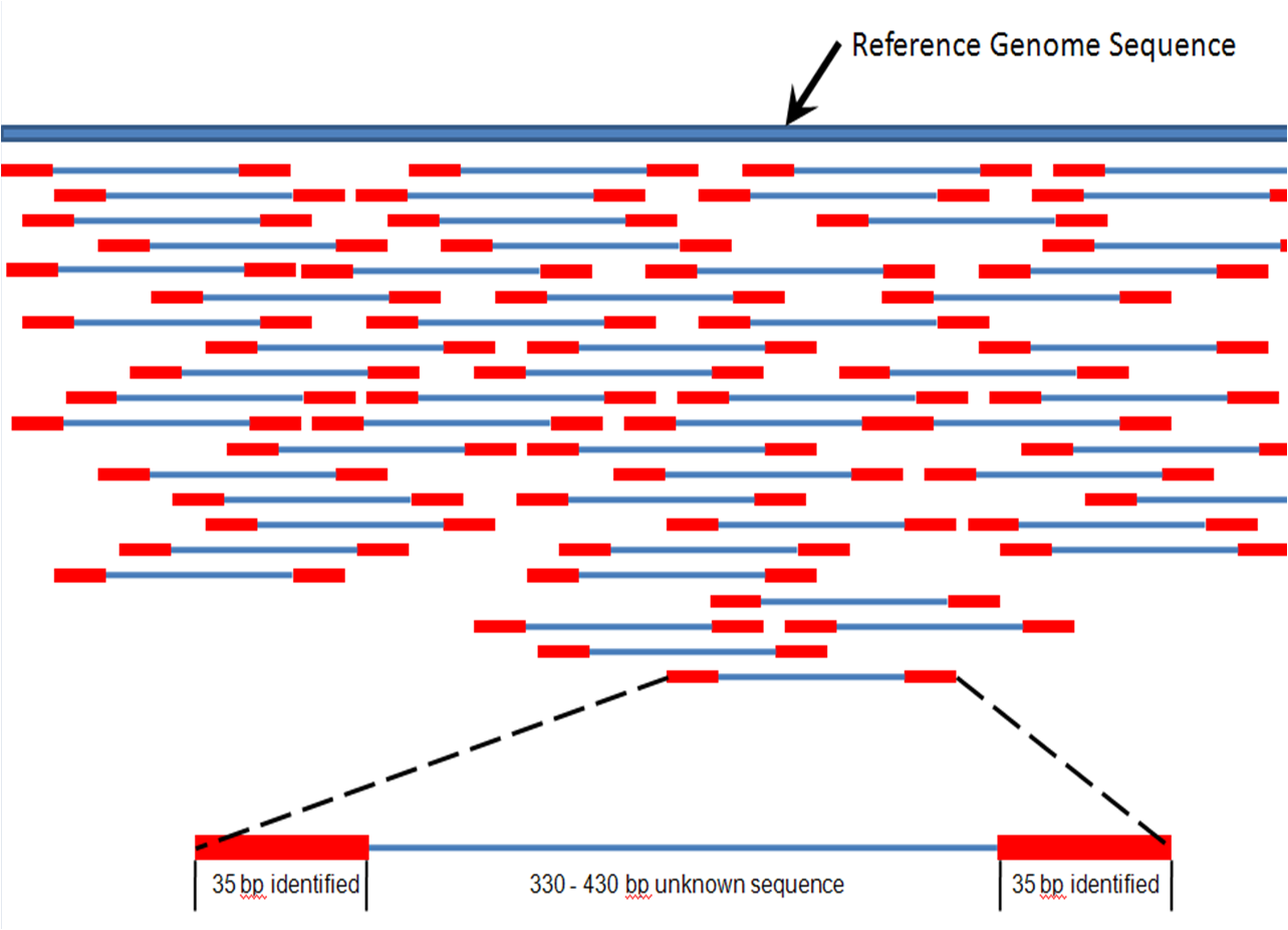 | ||
|
|
||
|
|
||
| ## 2. Reads mapping purposes | ||
|
|
||
| Read mapping techniques are used for several purposes. | ||
| Some examples: | ||
|
|
||
| 1) To evaluate the quality of an assembly (or to compare different methods used to assemble your reads). Read mapping can help identifying problematic areas in your assembly process. Indeed, statistics are necessary but might not be sufficient to evaluate the quality of your assembly. | ||
|
|
||
| To assess the quality of an assembly we can eg. to look at: | ||
| - the coverage regularity (ex: some repeated regions might have increased coverage) | ||
| - the coverage at the beginning and end of scaffolds - is it good enough? | ||
| - are there positions where pileup of reads show polymorphism? | ||
| - ... | ||
|
|
||
| 2) Assembly polishing software such as `pilon` and `reapr` use mapped reads to identify potential positions where the assemblies should be improved. It is good to visualize what information they are using. | ||
|
|
||
| Assembly polishing softwares can eg. use variation in coverage, wrong read pairs orientation, discrepancy between expected insert size and actual insert size obtained from read mapping (ie. longer than expected) to improve assembly. | ||
|
|
||
| 3) To identify SNPs: some methods use reads mapping against a reference genome to identify and type variants/SNPs (e.g. [snippy](https://github.com/tseemann/snippy)) | ||
|
|
||
| ## 3. Practical: mapping reads to the assembly obtained from the same reads. | ||
|
|
||
| We have assembled reads using `Bifrost pipeline`. The data for today's practical are found on SAGA in `/cluster/projects/nn9305k/tutorial/20210412_mapping_visualization/mapping_practical` | ||
|
|
||
| Description of the files in this folder: | ||
| - the raw_reads: `MiSeq_Ecoli_MG1655_50x_R{1,2}.fastq.gz` | ||
| - the trimmed-reads: `MiSeq_Ecoli_MG1655_50x_{R1,R2,S}_concat_stripped_trimmed.fq.gz` | ||
| - the assembly (polished with Pilon, output during prokka annoation): `MiSeq_Ecoli_MG1655_50x.fna` (fasta format) | ||
|
|
||
| Mapping can be done either with raw reads or trimmed reads. If you are interested to see if there are positions with SNPs, it is easier to use trimmed-reads (avoiding the visualization noise due to the presence of adapters) | ||
|
|
||
| To map reads, we use the [bwa mem] option from [bwa tools] software. | ||
|
|
||
| NB: Convention: means `<change_me>` | ||
|
|
||
|
|
||
| _**PRACTICAL EXERCISE:**_ | ||
|
|
||
| In your `home` directory make a directory for today's work | ||
| and a folder called `mapping` where you will **copy** the input files | ||
|
|
||
| ```bash | ||
| cd <home> | ||
| mkdir mapping | ||
| cd mapping | ||
|
|
||
| rsync -rauPW /cluster/projects/nn9305k/tutorial/20210412_mapping_visualization/mapping_practical/* . | ||
| ``` | ||
|
|
||
|
|
||
| You can look at the file content e.g. (one reads-file, the assembly file): | ||
| ```bash | ||
| head MiSeq_Ecoli_MG1655_50x.fna | ||
| gunzip -cd MiSeq_Ecoli_MG1655_50x_S_concat_stripped_trimmed.fq.gz | head | ||
| ``` | ||
|
|
||
| The mapping tool called `bwa tools` which is installed in the **Bifrost pipeline** conda environment. | ||
|
|
||
| Here are options for performing the mapping: | ||
| 1. You can use the raw_reads for mapping | ||
| 2. You can use the trimmed reads for mapping | ||
| 3. You can perform 2 mapping rounds with raw_reads and trimmed reads (2 times). This might be interesting if you want to look at the effect of trimming or not on the mapping visually. | ||
|
|
||
| For the tutorial, you will chose one solution 1 or 2. (Solution 3 is if you are curious and want to repeat the exercise) | ||
|
|
||
| You will ask for interactive ressources in saga and activate the `bifrost` environment. (We use the queue for testing purposes: devel) | ||
|
|
||
| ```bash | ||
| srun --account=nn9305k --mem-per-cpu=4G --cpus-per-task=2 --qos=devel --time=0:30:00 --pty bash -i | ||
| conda activate bifrost | ||
| ``` | ||
|
|
||
| To map the reads to an assembly/reference we need to: | ||
| 1) Index the reference: we are in this case using the assembly as reference | ||
|
|
||
| ```bash | ||
| bwa index <reference.fna> | ||
| ``` | ||
|
|
||
| 2) We map the reads (attribute the position of the reads according to the index) and sort the mapped reads by index position | ||
|
|
||
| NB: Here `-` means that the output of the pipe `|` is used as input in samtools. And `\` is used to indicate that your code (instructions) continues on the next line | ||
|
|
||
| - for paired reads (PE) or paired trimmed reads: | ||
|
|
||
| ```bash | ||
| bwa mem -t 4 <reference.fna> <in1:read1.fq.gz> <in2:read2.fq.gz> \ | ||
| | samtools sort -o <out:PE_mapped_sorted.bam> - | ||
| ``` | ||
|
|
||
| - If you used trimmed reads (follow below) you also have unpaired reads (called S here) that we can map as such: | ||
|
|
||
| ```bash | ||
| bwa mem -t 4 <reference.fna> <in:S_reads.fq.gz> \ | ||
| | samtools sort -o <out:S_mapped_sorted.bam> - | ||
| ``` | ||
|
|
||
| - You can merge merged the paired trimmed reads and S reads as such: | ||
|
|
||
| ```bash | ||
| samtools merge <out:all_merged.bam> <in1:S_mapped_sorted.bam> <in2:PE_mapped_sorted.bam> | ||
| ``` | ||
|
|
||
| - Now we need to be sure merged reads are still sorted by index: we resort | ||
|
|
||
| ```bash | ||
| samtools sort -o <out:final_all_merged.bam> <in:all_merged.bam> | ||
| ``` | ||
|
|
||
| **OPTIONAL** | ||
|
|
||
| NB: Some software like `Pilon` need an updated index after merging bam files). You do that by running: | ||
|
|
||
| ```bash | ||
| samtools index <final_all_merged.bam> | ||
| ``` | ||
|
|
||
| ## 4. Understanding the mapping file format: the [sam/bam file format] | ||
|
|
||
| `.bam` files are in a compressed binary format. We need to transform the `.bam` (to a `.sam` file) to be able to see how mapped-reads are represented in the file. | ||
|
|
||
| Also have a look at [Samtools article] and at [Samtools manual] | ||
|
|
||
|
|
||
| _**PRACTICAL EXERCISE:**_ | ||
|
|
||
| To decompress: chose f.eks. `PE_mapped_sorted.bam` that we did in the first step: | ||
|
|
||
| ```bash | ||
| samtools view -h -o <out.sam> <in.bam> | ||
| ``` | ||
| Look at your `.sam` file using: | ||
|
|
||
| ```bash | ||
| less <filename.sam> | ||
| ``` | ||
|
|
||
| ## 5. Looking at how the reads maps against the reference/assembly with [Samtools] `tview` module | ||
|
|
||
| - looking at the reads pileup with SAMtools | ||
| - use `-p <position>` if you want to see a specific position | ||
| - type `?` to view the navigation help while samtools is running | ||
| - type `q` to quit | ||
|
|
||
|
|
||
| _**PRACTICAL EXERCISE:**_ | ||
|
|
||
| ```bash | ||
| samtools tview <final_all_merged.bam> --reference <assembly> | ||
| ``` | ||
|
|
||
| ## Going further | ||
| Suggested next lesson: [Visualizing assembly and associated reads pileup with IGV](./Visualisation_assembly_reads_pileup_IGV.md) | ||
|
|
||
| You can also look here at the [Uio course] for more details or if you want to do things slightly differently. We reuse some of their [scripts](https://inf-biox121.readthedocs.io/en/2017/Assembly/practicals/Sources.html). | ||
|
|
||
| [Uio course]:https://inf-biox121.readthedocs.io/en/2017/Assembly/practicals/03_Mapping_reads_to_an_assembly.html | ||
|
|
||
| [bwa mem]:http://bio-bwa.sourceforge.net/bwa.shtml | ||
|
|
||
| [bwa tools]:http://bio-bwa.sourceforge.net/ | ||
|
|
||
| [Samtools article]:https://academic.oup.com/bioinformatics/article/25/16/2078/204688 | ||
|
|
||
| [Samtools manual]:http://www.htslib.org/doc/samtools.html | ||
|
|
||
| [Samtools](http://www.htslib.org/doc/samtools.html) | ||
This file contains hidden or bidirectional Unicode text that may be interpreted or compiled differently than what appears below. To review, open the file in an editor that reveals hidden Unicode characters.
Learn more about bidirectional Unicode characters
| Original file line number | Diff line number | Diff line change |
|---|---|---|
| @@ -0,0 +1,15 @@ | ||
| # Transfering files between server and PC or to another server ? | ||
|
|
||
| ## scp | ||
|
|
||
|
|
||
| ## rsync | ||
|
|
||
|
|
||
| ```bash | ||
| # transfering from SAGA | ||
| rsync -rauPW <user_name>:<source_folder> <destination_folder> | ||
| ``` | ||
|
|
||
|
|
||
| ## filezilla |
Add this suggestion to a batch that can be applied as a single commit.
This suggestion is invalid because no changes were made to the code.
Suggestions cannot be applied while the pull request is closed.
Suggestions cannot be applied while viewing a subset of changes.
Only one suggestion per line can be applied in a batch.
Add this suggestion to a batch that can be applied as a single commit.
Applying suggestions on deleted lines is not supported.
You must change the existing code in this line in order to create a valid suggestion.
Outdated suggestions cannot be applied.
This suggestion has been applied or marked resolved.
Suggestions cannot be applied from pending reviews.
Suggestions cannot be applied on multi-line comments.
Suggestions cannot be applied while the pull request is queued to merge.
Suggestion cannot be applied right now. Please check back later.
There was a problem hiding this comment.
Choose a reason for hiding this comment
The reason will be displayed to describe this comment to others. Learn more.
refer to a page with rsync
Uh oh!
There was an error while loading. Please reload this page.
There was a problem hiding this comment.
Choose a reason for hiding this comment
The reason will be displayed to describe this comment to others. Learn more.
This page needs to be made. Removed this part - made a link (commented above) so has to be written