A repo to keep track of my understanding of some CS fundamentals. I will be adding notes and implementations where applicable.
I hope that this will eventually function as an all-in-one reference and learning page for others.
| Algorithm | Best case | Average case | Worst case | Stable | In place | Code | Remarks |
|---|---|---|---|---|---|---|---|
| Selection sort | n2 | n2 | n2 | Yes | Yes | - | Can be useful where auxiliary memory is limited |
| Insertion sort | n | n2 | n2 | Yes | Yes | - | Used for small or partially-sorted arrays |
| Bubble sort | n | n2 | n2 | Yes | Yes | - | Rarely useful; use insertion sort instead |
| Counting sort | n + k | n + k | n + k | Yes | Yes | - | Useful for when range of values each item can take is small |
| Merge sort | n log n | n log n | n log n | Yes* | No* | Python | - |
| Quick sort | n log n | n log n | n2 | No* | Yes* | Python | Worst case is rare |
| Heap sort | n log n | n log n | n log n | No | Yes | Python | - |
* Further information can be seen in the sections dedicated to each sort.
| Tree type | Worst: | Search | Insert | Delete | Avg: | Search | Insert | Delete |
|---|---|---|---|---|---|---|---|---|
| BST | O(n) | O(n) | O(n) | O(log n) | O(n) | O(n) | ||
| AVL | O(log n) | O(log n) | O(log n) | O(log n) | O(log n) | O(log n) | ||
| Red-black BST | O(log n) | O(log n) | O(log n) | O(log n) | O(log n) | O(log n) | ||
| Binary heap | O(n) | O(log n) | O(log n) | O(n) | O(1) | O(log n) |

To fill
- Trees in which each node has two or fewer children
- An extension of a linked list, where each node can be linked to two children rather than one (a linked list could be considered a "unary tree")
- The root is the single node at the top
- Branches connect nodes
- Nodes at the bottom (pointing to no other nodes) are called leaves
- Number of nodes = number of branches + 1
- The depth of a node is the number of branches from the node to the root (i.e. above)
- The height of a node is the number of branches from the node to its deepest descendant leaf
- The tree height is the number of branches from the root to the deepest leaf
- Largest number of nodes a binary tree can have if it has height n is 2n+1 - 1
- i.e. a tree of height 5 can have at most 25+1 - 1 = 26 - 1 = 64 - 1 = 63 nodes
class Node:
    """Define a node in a binary tree.
    """
    def __init__(self, value=None, left=None, right=None):
        self.value = value # information that is being stored in the tree
        self.left = left   # the left child (subtree)
        self.right = right # the right child (subtree)

    def __str__(self):
        return str(self.value)
| Root | No. branches | Leaves | Depth of node 7 | Height of node 7 | Tree height |
|---|---|---|---|---|---|
| 2 | 8 | 2, 5, 11, 4 | 1 | 2 | 3 |
- A full binary tree is a binary tree in which each node has exactly zero or two children
- A full binary tree will always have an odd number of nodes: 2 or 0 children for each node, plus the root

- A complete binary tree is a binary tree in which every level, except possibly the last, is completely filled and all nodes are as far left as possible

- A tree can be full but not complete and a tree can be complete but not full
- Traversal -> traverse all -> visit the whole tree and find all of its data
- Traversing a tree can be done pre-order (red), in-order (yellow) or post-order (green)

| Method | Order of nodes |
|---|---|
| Pre-order (red) | F,B,A,D,C,E,G,I,H |
| In-order (yellow) | A,B,C,D,E,F,G,H,I |
| Post-order (green) | A,C,E,D,B,H,I,G,F |
def traverse_pre_order(tree):
    """Traverse an input tree pre-order.
    """
    if tree:
        print(tree.getRootVal())
        traverse_pre_order(tree.getLeftChild())
        traverse_pre_order(tree.getRightChild())

def traverse_in_order(tree):
    """Traverse an input tree in-order.
    """
    if tree:
        traverse_in_order(tree.getLeftChild())
        print(tree.getRootVal())
        traverse_in_order(tree.getRightChild())

def traverse_post_order(tree):
    """Traverse an input tree post-order.
    """
    if tree:
        traverse_post_order(tree.getLeftChild())
        traverse_post_order(tree.getRightChild())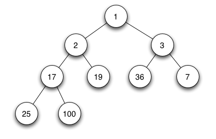
print(tree.getRootVal())- A binary tree where, for every node, all children in the left sub-tree contain smaller values and all children in the right sub-tree contain larger values
- BSTs therefore cannot have duplicate elements

- For best performance a BST should be well-balanced (i.e. as much as possible, the left and right branches at a particular position are "filled up" at each level without gaps)
- Essentially, we want it to be complete
- The time taken to find a node will be proportional to the node's depth
- Therefore deeper trees will have longer worst case search runtimes
- If the tree is complete (or at least balanced) then the depth of the tree will be approximatel equal to log2(n) and so the runtime will be O(log n)
- The worst case scenario for searching a BST is a "maximally unbalanced tree" i.e. where the BST gets reduced to a simple linked list. In this case the runtime goes to O(n)
- The simplest way to construct a BST is to initialise it with a single root node and repeatedly insert numbers into the tree
- To maintain the BST property, there will only ever be one position in which a node can be inserted
- Somewhat unintuitively, if you add pre-sorted data into a BST, it will have maximal inefficiency, O(n)

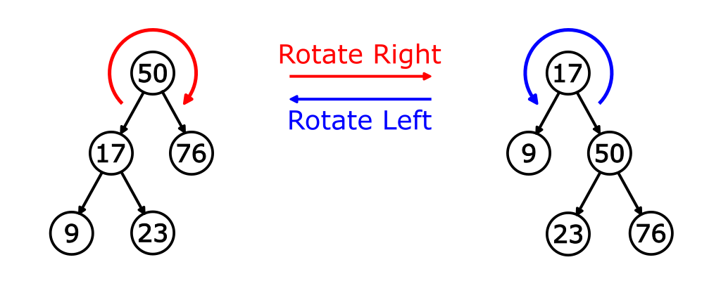
- A tree rotation is an operation on a binary tree that changes the structure of the tree without affecting the order of the elements (in-order traversal)
- It is used to balance out two branches of different depths
- One node gets shifted up, one node shited down and other nodes may be connected to different parents
- They are very useful for balancing trees for performance
- It may be easier to think of them as "clockwise" (right) and "anticlockwise" (left) rotations
- It doesn't matter whether the top node in a rotation has parents
- Rotations can therefore be used at any level of a tree

- AVL trees are self-balancing trees that, when adding nodes, look for a chain of 3 nodes that are singly linked
- Appropriate rotations are applied when this happens to turn those nodes into a parent and two children
- AVL trees are good at balancing, but often require multiple rotations per operation (insertion/deletion)
- Perfect for when the tree will be created only once and not modified, but the data will be accessed often
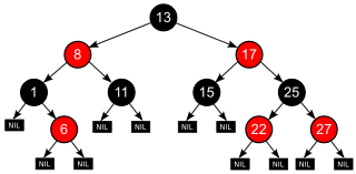
- Red-black trees are also self-balancing and are less strict than AVL trees
- The result is a slightly slower average lookup, but faster insertion and deletion
- All nodes in the tree are either red or black (surprisingly)
- Newly inserted nodes are always red; depending on the surrounding nodes they will be rotated or repainted according to different contraints
- The result will not be a perfectly balanced tree
- However, it will have a guaranteed worst case runtime of O(log n) for searching, insertion and deletion
- It is guaranteed to have a maximum height of 2 log(n + 1)
- Any path from a given node to any of its descendant NIL nodes goes through the same number of black nodes
- Good for when data will be regularly modified and accessed
- Used when you will need to get the most important item in a data structure (imagine patients checking into A&E; it doesn't work using FIFO)
- Three basic operations:
insert(i,p)- add an element i with priority ppop()- remove and return the item with the highest prioritypeek()- look at the value of the highest priority element without changing the queue
- The best runtime is achieved by organizing data in a binary tree format, giving a runtime of O(log n) vs O(n) in other implementations

A max heap and min heap, respectively
- A binary heap is considered the best structure for priority queues
- Binary heaps are binary trees where the value of each node must be greater than or equal to the values of its left and right children (for a max heap; it is the other way round for a min heap)
- As a result, the highest priority item is always at the top of the heap
- A binary heap is complete
- A node with index n conventinally has child nodes of 2n and 2n+1; i.e. the top node has index (not priority) 1 and its children have index 2 and 3
- To insert an item:
- Add it to the first open position in the binary heap
- Bubble it up to the top until there are no elements above it with a higher priority (i.e. it is at the root or below a higher priority node)
- The best way to construct a heap is to:
- Randomly insert all values in an arbitrary order to get a random heap
- "Max heapify" by bubbling up the nodes at each position, starting at the leaves and working up
- Constructing a binary heap in this way takes a runtime of O(n)
To fill
To fill
To fill
To fill
To fill
First divide the list into the smallest unit (1 element), then compare each element with the adjacent list to sort and merge the two adjacent lists. Finally all the elements are sorted and merged.
- A divide-and-conquer algorithm
- Stable (in most implementations)
- Does not sort in-place (in most implementations - see block merge sort for in place)
| Best case | Average case | Worst case |
|---|---|---|
| O(½ n log n) | O(n log n) | O(n log n) |

Python, using pointers (reduced space complexity)
David Taylor: Algorithms with Attitude (fantastic explainer video on optimisations etc.)
Select a 'pivot' element from the array and partition the other elements into two sub-arrays, according to whether they are less than or greater than the pivot. The sub-arrays are then sorted recursively. This can be done in-place, requiring small additional amounts of memory to perform the sorting.
- A divide-and-conquer algorithm
- Not stable for efficient implementations
- Does sort in-place
| Best case | Average case | Worst case |
|---|---|---|
| O(n log n) | O(2n ln n) | O(½n2) |

Heapsort divides its input into a sorted and an unsorted region, and it iteratively shrinks the unsorted region by extracting the largest element from it and inserting it into the sorted region.
- Put all the numbers into an array in an arbitrary order.
- Organize the binary heap one element at a time by repeatedly swapping larger children with smaller parents.
- Switch the root of the heap with the node furthest down.
- Remove what was previously the root from the heap. Store it as the smallest of the already sorted numbers.
- Repeat the previous three steps until the heap is empty. The list of stored numbers will be sorted.
- Utilises a binary heap
- Not stable
- Does sort in-place
| Best case | Average case | Worst case |
|---|---|---|
| O(n log n) | O(n log n) | O(n log n) |

To fill
To fill
Recursion is a method of solving a problem where the solution depends on solutions to smaller instances of the same problem. The same problems can be solved iteratively, but this would involve identifying the indexes and redefining them at each stage. Recursion allow you to solve such a problem without doing so.
The power of recursion evidently lies in the possibility of defining an infinite set of objects by a finite statement. In the same manner, an infinite number of computations can be described by a finite recursive program, even if this program contains no explicit repetitions.
While often easier to define, one drawback of recursion is that memory usage can be harder to control.
Recursive functions call on themselves until they reach a defined base case, where the stack of calls then begins to "unravel".
def binary_search(A, item):
    if len(A) == 0:
        return False
    else:
        middle = len(A) // 2
        if A[middle] == item:
            return True
        if item < A[middle]:
            return binary_search(A[:middle], item)
        else:
return binary_search(A[middle + 1:], item)To fill
To fill