- Introduction
- Why Classification?
- What is Classification?
- What are the types of Classification algorithms?
- K-Nearest Neighbors Classification
- Support Vector Machine
- Biomedical Applications
- Conclusion
The explosive growth of technology in bioinformatics yields new biological datasets, which presents both unique opportunities and challenges. The accumulation of new sequencing, protein structure, and 3-D genome interaction data has revolutionized our understanding of the human body. Amid this abundance of information, the extraction of meaningful insights rely on effective organization and analysis. This is where classification comes into play, a group of supervised machine learning models that can be used to categorize and decipher patterns in biological data. This paper will navigate the current landscape of classification algorithms by exploring different types of machine learning algorithms and discussing their powerful applications to biomedical problems.
Let's explore a simple scenario to motivate the importance of classification in machine learning.
You are given a task to categorize a given object as a fruit or a vegetable.

This single object is a corn, and it is a trivial task to place this into the vegetable category.
Now consider this task: you are given a task to categorize the 1 million objects in this wagon as a fruit or a vegetable.

What if the objects you are asked to classify are pictures of tumors?
Determining the malignancy of the tumor is critical for survival.
This report will discuss how classification algorithms can automate and accelerate this process of categorization tremendouly.
Classification is a supervised machine learning model that identifies the category that an observation belongs to.
- Logistic Regression
- Random Forest
- k-Nearest Neighbor
- Neural Network
- Support Vector Machines
Here, we will briefly discuss three powerful classification algoriths: k-Nearest Neighbor, Neural Network, and Support Vector Machines.
To build a stronger intuition about k-Nearest Neighbor and Support Vector Machines, please see their respective sections below.
The k-Nearest Neighbor (k-NN) method categorizes a new data point based on the k-nearest neighbors around that data point. For example, if k = 11, we will categorize the new data point based on the majority category of the 11 nearest points near it.
STEPS
1. Prepare the data containing various data points with known classes or labels
2. Introduce a brand new data point (the unknown vegetable) that you want to categorize based on its characteristics.
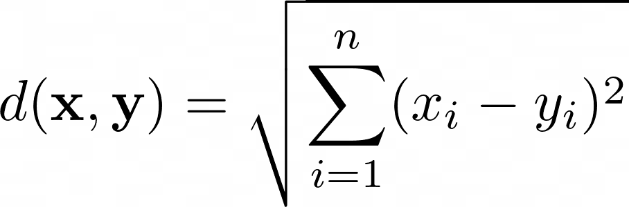
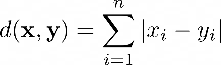
3. The k-NN algorithm identifies the k neighbors closest to the new data point based on similarity scores (using metrics such as Euclidean or Manhattan distancing).
4. Classify the new data point as the most common label among the k nearest neighbors.
Note: It is important to plot the validation curve in order to determine the optimal value for k.
From:
KNN Overview, StatsQuest Video
See the K-Nearest Neighbors section for more details
A neural network consists of an input layer, n hidden layers, and an output layer. Each node in the layer has a specific weight and bias attached to them, and all layers are connected. As we train the model, we adjust the weight and bias of the nodes, through techniques like gradient descent, so that it results in a more accurate model.
STEPS
1. Preprocess and prepare the data.
2. Choose a type of neural network that suits your needs. (i.e. convolutional neural network)
3. Design the architecture of the model. How many layers do we want? What types of layers do we want? How many nodes per layer?
4. Define the loss function (i.e. cross-entropy loss ), which measures the performance of the classification model. Set up the optimizer (i.e. Adam).
5. The optimizer will adjust learning rates for each parameter, gradually improving the performance of the model by minimizing the loss function. This will be the basis for our learning.
6. Feed the training data into the model.
Have proper measures to prevent overfitting. Simplifying the neural network architecture or incorporating regularization in each node may help prevent overfitting.
Example from TensorFlow:
model.compile(optimizer='adam',
              loss=tf.keras.losses.SparseCategoricalCrossentropy(from_logits=True),
              metrics=['accuracy'])

history = model.fit(train_images, train_labels, epochs=10,
                    validation_data=(test_images, test_labels))
7. Once the model is ready, introduce new unknown data and make a prediction
Note: Use TensorFlow for Neural Network implementation

From:
Convolutional Neural Networks, Adam, Cross Entropy Loss, Types of Neural Networks, TensorFlow Example
Support Vector Machines (SVMs) classify data points by finding the most optimal decision boundary. The main aim of SVM is to find a hyperplane that maximizes the distance from data points in different categories. Incorporating kernel functions, which map points to a higher dimensions, can make data points more separable. Overall, SVMs play an important role in separating data for classification.
STEPS
1. Preprocess and prepare the data
2. Choose a kernel (i.e. linear, polynomial, sigmoid, Gaussian Radial Basis Function, etc) based on the type of data being used
3. Tune the kernel hyper parameters (i.e. gamma RBF)
4. Set up the SVM model (i.e. Scikit-learn)
5. Train the model using the .fit method
svm_cv.fit(X_train,y_train)
6. Assess the performance using accuracy, recall, etc. Adjust hyper parameters if unsatisfactory
7. Once the model is ready, introduce new unknown data and run it through the model

From:
SVM Overview, StatsQuest Video
See the SVM section for more details
The k-Nearest Neighbor (k-NN) method is like asking your closest neighbors for advice. Imagine a scenario in which you have an unknown vegetable and you are trying to figure out what type of vegetable it is. You look at the labeled vegetables that your neighbors have, compare them, and decide based on the most similar ones.
The training process of the KNN classification algorithm is fairly straightfoward. The algorithm stores the entire data set to memory while keeping track of distances (for example Euclidean Distance).
In python we can calculate these using numpy or scipy
Euclidean Distance Formula:
Manhattan Distance Formula:
Near Neighbor Search in High Dimensional Data
It is important to choose the most optimal k-value, as it will be essential for managing outliers/noise in the dataset. When k=1, the model makes predictions based solely on the closest neighbor to a data point. This can cause the model to capture noise or outliers, leading to overfitting because it's overly tailored to the training data. However, if the k value is too large, it can lead to oversimplification of the model and the creation of overly generalized boundaries.
Although there are various ways to compute the optimal k (i.e. square root of the total # of datapoints ), the most consistent approach will be the k elbow curve method.
import pandas as pd
import numpy as np
from sklearn.model_selection import train_test_split
from sklearn.neighbors import KNeighborsClassifier
import matplotlib.pyplot as plt

data = pd.read_csv(‘KNN_Project_Data) \\ read data

error_rate = [] \\keep track of error rates through various k values
for i in range(1,40):
 knn = KNeighborsClassifier(n_neighbors=i)
 knn.fit(X_train,y_train)
 pred_i = knn.predict(X_test)
 error_rate.append(np.mean(pred_i != y_test))

plt.figure(figsize=(10,6)) //plot example
 // ... include color implementations, etc.
plt.title(‘Error Rate vs. K Value’)
plt.xlabel(‘K’)
plt.ylabel(‘Error Rate’)
By keeping track of the error rates and the k values, we will be looking at which k value has the lowest error rate. By doing so we can prevent over/under fitting.
For example:

The optimal k value will be 20 as it has the lowest error rate.
Elbow Method

When we introduce a new data point we will calculate the distances from the new data point to the others using the chosen distance metric. Then we can sort the calculated distances in ascending order based on distance values. This way, we can look at the top k rows for the closest k neighbors. Ultimately, we can label the new data point based on the most common label among the k closest neighbors.
There are several limitations for the k-nearest neighbor model. The run time growns linearly with the size of the training data, meaning it can be extremely extensive with big data sets. This also means that it will take up a significant amount of memory as we are storing all the points.
One feature that can possibly limit the model is the neccesity of the optimal k value. Sub-optimal k values can result in an overfit or underfit model that is sensitive to noise in the dataset.
When running k-nearest neighbor on an unbalanced dataset, the accuracy of the model is likely to be low. This is due to the fact that the majority can dominate the decision of the model, which causes the minority have a higher chance of being misclassified.
These limitations reveal the need for careful consideration and preprocessing of data before applying the k-NN algorithm. Addressing these issues by optimizing the k value can improve the model's effectiveness in real-world applications. Additionally, exploring alternative algorithms or methods that can handle large datasets more efficiently might offer solutions to the challenges k-NN faces.
Support Vector Machines aim to classify labeled data into two classes. Imagine you are looking at a soccer field with two groups: players wearing red jerseys and players wearing blue jerseys. The SVM finds a hyperplane that separates these two groups of players based on their jersey color. It finds a hyperplane that maximizes the distance between the closest players to the line. These players would be the support vectors and other players would not play a role in the position and orientation of the hyperplane. SVM also allows for misclassifications which is important for generalization.
Support Vector Machines are implemented by creating a hyperplane to separate the labeled data into two groups. Groups are not always linearly separable so we may need to apply a transformation to make separation possible. This transformation is called a kernel, which I discuss further below. Let us now take a look at how to implement an SVM in code. Code Source
import numpy as np
import matplotlib.pyplot as plt
from matplotlib.colors import ListedColormap
import pandas as pd
from sklearn.model_selection import train_test_split
from sklearn.preprocessing import StandardScaler
from sklearn.svm import SVC
from sklearn.metrics import confusion_matrix, accuracy_score

dataset = pd.read_csv('dataset.csv')

// spliting the data into X and Y
X = dataset.iloc[:, [2, 3]].values
y = dataset.iloc[:, 4].values

// split data into training and test sets
X_train, X_test, y_train, y_test = train_test_split(X, y, test_size = 0.25, random_state = 0)


// scaling our data values to normalize them
sc = StandardScaler()
X_train = sc.fit_transform(X_train)
X_test = sc.transform(X_test)

// use the 'rbf' kernel, a non-linear transformation that helps us fit the SVM
classifier = SVC(kernel = 'rbf', random_state = 0)
classifier.fit(X_train, y_train)

// run SVM on test data to see predictions
y_pred = classifier.predict(X_test)

// get accuracy
cm = confusion_matrix(y_test, y_pred)
print(cm)
accuracy_score(y_test,y_pred)

// visualize the data
X_set, y_set = X_test, y_test
X1, X2 = np.meshgrid(np.arange(start = X_set[:, 0].min() - 1, stop = X_set[:, 0].max() + 1, step = 0.01),
                     np.arange(start = X_set[:, 1].min() - 1, stop = X_set[:, 1].max() + 1, step = 0.01))
plt.contourf(X1, X2, classifier.predict(np.array([X1.ravel(), X2.ravel()]).T).reshape(X1.shape),
             alpha = 0.75, cmap = ListedColormap(('red', 'green')))
plt.xlim(X1.min(), X1.max())
plt.ylim(X2.min(), X2.max())
for i, j in enumerate(np.unique(y_set)):
    plt.scatter(X_set[y_set == j, 0], X_set[y_set == j, 1],
                c = ListedColormap(('red', 'green'))(i), label = j)
plt.title('SVM (Test set)')
plt.xlabel('Age')
plt.ylabel('Estimated Salary')
plt.legend()
plt.show()
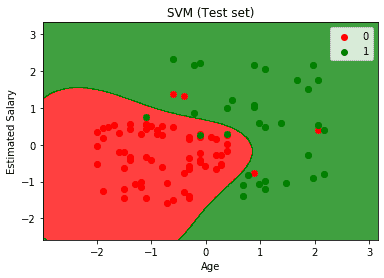
One of the main kernels that we can use is the rbf kernel, a non-linear kernel. This kernel projects vectors to an infinite dimensional space to help with separability. Other kernels can also be used depending on the data to separate two classes of data. For example, the linear kernel is used when the data is linearly separable. Kernels
Some limitations include the lack of interpretability (what makes a dataset belong to one class vs another) and difficulty in tuning the hyperparameters C and gamma. The C hyperparameters determine the tradeoff between correct classification and maximizing the margin. The gamma parameter determines the radius around the supper vectors where points in that radius will influence the hyperplane. Limitations
Machine learning is transforming biomedical sciences. Novel technologies are producing biological/medical datasets of unprecedented scale and resolution. As bioinformaticians, our role is to leverage this data to yield insights into complex biological systems and/or improve diagnosis and treatment.
Here, we will discuss three key applications of classification to biomedical sciences.
1. Early Detection / Disease Diagnosis
2. Disease Monitoring
3. Functional Genomics
Classification algorithms can assist in early detection and disease diagnosis. These machine learning tools have the potential to accelerate decision-making of disease diagnosis by automating visual examinations, perhaps to flag abnormalities. Expediting this process while maintaining accuracy can enable early detection of conditions such as skin cancer, in which early diagnosis improves prognosis for survival tremendously.
From: ML and Medical Diagnosis
For example, classification algorithms can be applied to distinguish between Benign and Malignant tumors.
:max_bytes(150000):strip_icc():format(webp)/514240-article-img-malignant-vs-benign-tumor2111891f-54cc-47aa-8967-4cd5411fdb2f-5a2848f122fa3a0037c544be.png)
Let's explore a scenario in which a healthcare provider wants to classify a tumor based on an image. Based on several visual features of the tumor images, can we accurately catergorize the tumor as benign or malignant?
Khairunnahar et al. 2019, Informatics in Medicine Unlocked explores this question by implementing a logistic regression model for tumor classification. They utilize a labeled breast cancer diagnosis dataset with the following features: Radius, Texture, Perimeter, Area, Smoothness, Compactness, Concavity, Concave points, Symmetry and Fractal dimension. In their analysis, they create a logistic regression model that can predict tumor malignancy with 97.4249% accuracy. See ROC curve below:

Next, let's explore a scenario in which a bioinformatician wants to classify a tumor based on the cell's gene expression profiles. The phenotypes of various cells are governed by their gene expression patterns. These unique gene expression profiles can be leveraged to classify cell samples into malignant or benign categories.
Divate et al. 2022, cancers leverages a deep neural network to distinguish between 37 cancer types for a total of 2848 samples.
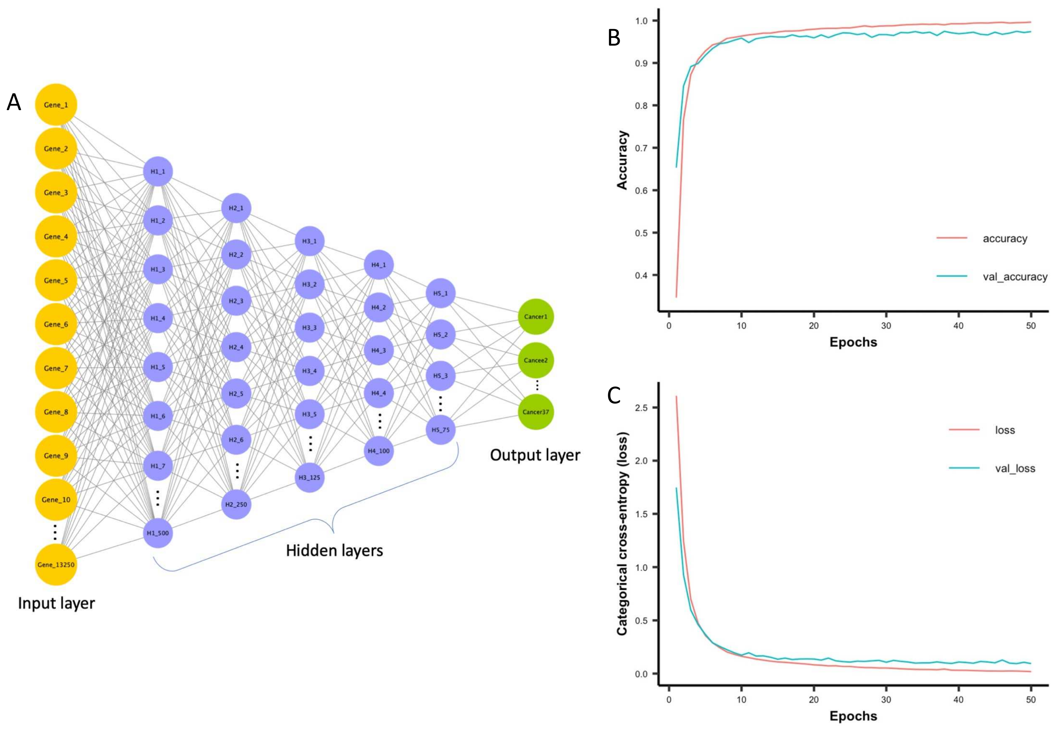
In this model, they utilize gene expression levels for 13,250 genes as input data to a neural network. Their model achieves a 97.33% overall accuracy on their testing data. Interestingly, they interpret the layers of the neural network to identify several gene signatures that can be used as biomarkers for determining the cancer's tissue of origin.
Classification algorithms can also improve disease monitoring by categorizing the severity of a condition. Monitoring key clinical variables for a disease and leveraging these machine learning models can potentially inform professionals of the direction of disease progression and help them make clinical decisions.
Jovel et al. 2021, Frontiers in Medicine applies many of the classification algorithms described in this paper to predict the survival of hepatitis patients based on blood tests that reflect liver function.
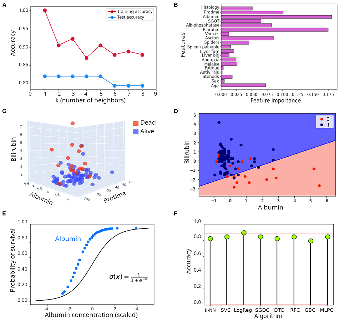
Notably, they implemented k-nearest neighbors, random forest, support vector machine, and logistic regression models to perform this classification task. Figure F above shows that the logistic regression model outperforms other models by achieving a 90% accuracy. Figure A displays that the k-nearest neighbors algorithm performed best with k = 1-5. Analyzing the importance of every feature in the random forest model, as shown in figure B, shows that Albumin, Bilirubin, and Protime levels (all proteins or compound found in the liver) are the most important features in predicting the survival outcome of hepatitis patients. Indeed, plotting the data as a scatter plot with these three measurements on the axes (figure C) show that these features separate the two categories of patients in 3-dimensional space. Lastly, figure D shows the decision surface used by the logistic regression model, reflecting it's effectiveness in separating patients in the two survival outcomes.
Although classification tasks are less common in functional genomics, there are certainly some powerful applications of classification algorithms for genomic annotation.
Amariuta et al. 2019, AJHG created a regularized logistic regression model (elastic net) to predict transcription factor occupancy at binding motifs based on local epigenomic features.

Here, ChIP-seq data is used as the cellular truth to train the logistic regression model. Hundreds of local epigenetic features, including open chromatin and H3K4me1, are used as variables to predict the probability of TF occupancy at nuceotide resolution. This models achieves a average AUPRC higher than state-of-the-art approaches to predict TF binding. Integration with genome-wide association study (GWAS) data shows that regulatory elements identified by IMPACT explains a large portion of the heritability of complex diseases such as rheumatoid arthritis.
- Classification is a powerful group of supervised machine learning models that can predict the categorical labels of input objects. Each of these classification algorithms introduced in this paper have their own advantages and limitations.
- Machine-learning is poised to transform biomedical sciences. We introduced three key applications of classification: disease diagnosis, disease monitoring, and functional genomics.
- The development of novel classification algorithm can potentially accelerate clinical decision-making, democratize disease diagnosis/monitoring, and propel therapeutic development.